
Smart meter data becomes useful when you stop treating it as a colourful chart and turn each interval into a cost. The goal is to identify the hours that repeatedly combine high consumption with an expensive tariff, then test whether those loads can be reduced, shifted, automated, or measured more closely.
For a flat-rate household, the costliest hours are usually the hours with the most imported energy. On a time-of-use tariff, the answer can be different: a smaller evening load at a high peak rate may cost more than a larger overnight load. Solar adds another layer because daytime consumption may replace low-value exports rather than full-price grid imports.
Short answer: export at least two to four weeks of interval data, attach the correct import rate to every interval, calculate
interval kWh x rate, and group the results by hour of day. Then separate recurring patterns from one-off events before changing appliances or tariffs.
What you need before you start
Collect these four items:
- Interval usage data from the retailer, distributor, utility portal, or meter-data service. In Australia, household smart meter data is commonly presented in 30-minute intervals, although the available interval and file structure depend on the provider.
- The actual tariff schedule from your current plan, including peak, shoulder, off-peak, controlled-load, and seasonal rules where applicable.
- The bill period and time zone, including any daylight-saving change within the analysis window.
- Context for major loads, such as EV charging, electric hot water, heating, cooling, pool pumps, batteries, or unusual occupancy.
Use at least 14 days when possible. A full billing period is better, and comparing similar seasons is better still. One day can reveal a clue; it cannot establish a reliable household pattern.
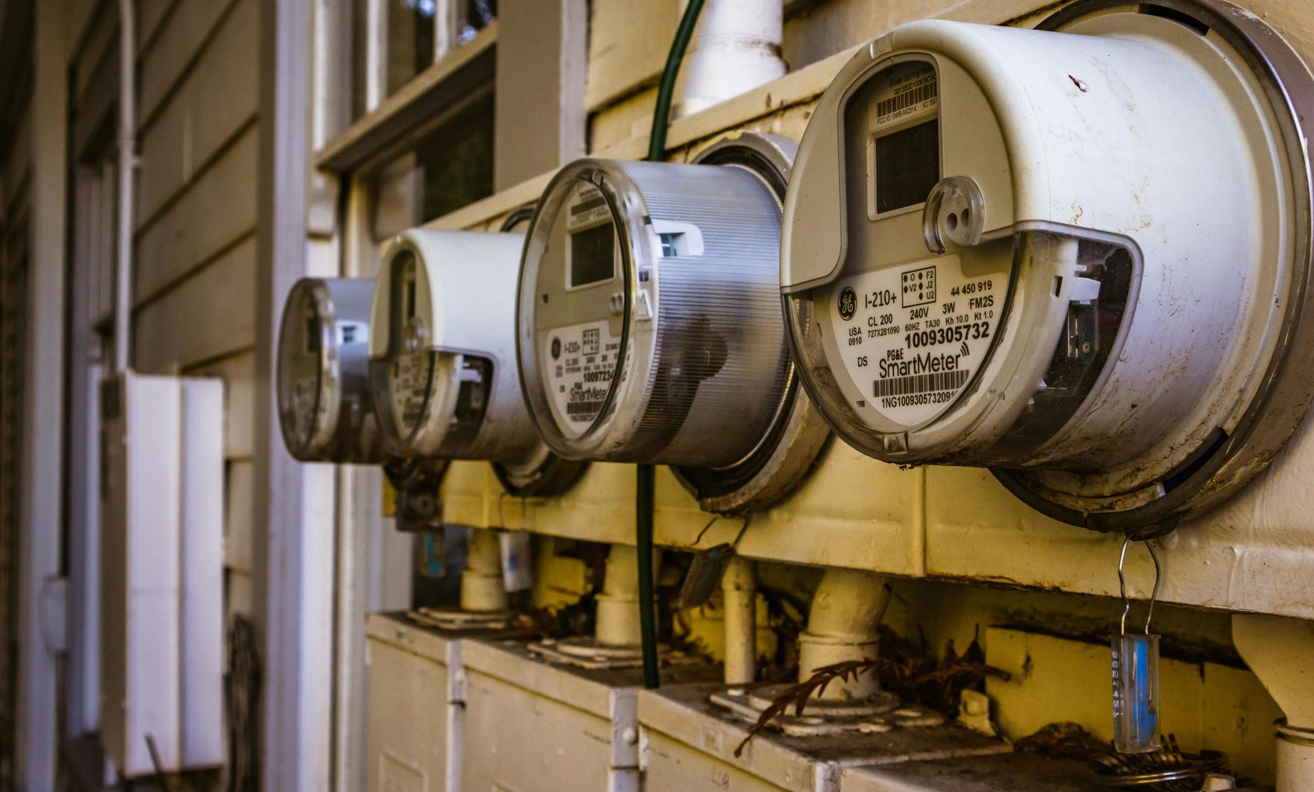
Utility smart meter data is usually the right starting point for bill analysis because it follows the billing boundary. A faster whole-home monitor becomes useful when the utility intervals are too coarse to identify the load behind a pattern.
First, understand the columns
The exact file varies, but useful interval data normally contains a timestamp and one or more energy values. Before calculating anything, identify what each value means.
| Field | What it should represent | Common mistake |
|---|---|---|
| Timestamp | Start or end of the interval in the stated time zone | Shifting every reading by one interval or mishandling daylight saving |
| Import energy | Energy drawn from the grid during the interval, usually kWh | Treating cumulative meter register data as interval usage |
| Export energy | Energy sent to the grid during the interval | Adding export to household consumption |
| Power | Rate of energy use at a moment or interval average, usually kW | Multiplying kW by the tariff without accounting for interval length |
| Quality flag | Actual, substituted, estimated, or missing data status | Treating estimated intervals as measured appliance behaviour |
| Register/channel | General usage, controlled load, import, export, or another stream | Combining channels billed at different rates |
The most important distinction is kW versus kWh. Power in kW describes how fast energy is being used. Energy in kWh is what most usage charges are based on. If your file contains average kW rather than interval kWh, convert it using the interval duration:
interval kWh = average kW x interval hours
For a 30-minute interval, multiply average kW by 0.5. For a 15-minute interval, multiply by 0.25.
Build an interval cost table
Create a spreadsheet with one row per interval and these columns:
| Column | Example logic |
|---|---|
| Date/time | Original timestamp converted to the correct local time |
| Date | Calendar date |
| Hour | Hour of day, such as 0 to 23 |
| Day type | Weekday or weekend; add public holiday if the tariff uses it |
| Import kWh | Meter-data import value |
| Export kWh | Meter-data export value, if solar is present |
| Tariff period | Peak, shoulder, off-peak, controlled load, or flat |
| Import rate | Rate that applies to that interval |
| Feed-in rate | Export credit that applies, if relevant |
| Import cost | import kWh x import rate |
| Export credit | export kWh x feed-in rate |
| Net variable cost | import cost - export credit |
Keep daily supply charges separate. They matter to the bill, but assigning them to a particular hour will not tell you which load to change. Demand charges also need their own analysis because they may depend on the highest kW during a defined window rather than total kWh.
A simple worked example
Assume these illustrative rates, not a market recommendation:
- peak import:
$0.55/kWh - off-peak import:
$0.22/kWh - solar feed-in credit:
$0.06/kWh
Now compare two intervals:
| Interval | Imported energy | Rate | Import cost |
|---|---|---|---|
| 6:00-6:30 pm | 0.70 kWh | $0.55/kWh | $0.385 |
| 1:00-1:30 am | 1.20 kWh | $0.22/kWh | $0.264 |
The overnight interval uses more energy but costs less. This is why sorting only by kWh can point you toward the wrong behaviour on a time-of-use plan.
Group cost by hour of day
Once every row has a calculated variable cost, build a pivot table or grouped summary:
- rows: hour of day;
- values: total import kWh, total import cost, total export kWh, and count of intervals;
- filters: weekday/weekend, month, season, and tariff period;
- optional value: average cost per day for that hour.
Sort by total cost, then by frequency. The most actionable hour is not necessarily the single largest spike. A moderate load that appears every weekday during the peak period can cost more over a month than one exceptional event.
A useful ranking table looks like this:
| Rank | Hour | Average daily import | Average daily variable cost | Pattern |
|---|---|---|---|---|
| 1 | 6-7 pm | High | Highest | Cooking, heating/cooling, hot water recovery |
| 2 | 7-8 pm | Medium-high | High | Dishwasher, dryer, entertainment, heating |
| 3 | 1-2 am | High | Medium | EV charging or controlled equipment at a lower rate |
| 4 | 3-4 am | Low but steady | Moderate over a month | Always-on load or scheduled equipment |
The values will differ by home. The point is to connect cost, timing, and repetition.
Read the shape, not just the total
Most households fall into a few recognisable patterns.
The evening peak stack
Usage climbs when occupants arrive home and cooking, heating or cooling, hot water, lighting, laundry, and entertainment overlap. On a time-of-use tariff, this can be the most expensive part of the day even when no single appliance looks excessive.
Best response: shift the dishwasher, dryer, EV charging, pool pump, or water heating outside the peak window before sacrificing necessary cooking or comfort.
The high overnight floor
Usage never drops as low as expected. Refrigeration, network equipment, electric hot water, pool equipment, pumps, standby loads, or an EV charge schedule may be responsible.
Best response: compare several quiet nights, then use a plug-in meter, circuit monitor, or controlled isolation process. Our guide to finding an always-on power load explains that workflow.
The morning rebound
Heating, hot water, kettles, cooking, and household preparation create a sharp morning rise. If the tariff's peak window includes that period, it may be costly; if not, it may simply be a visible but acceptable routine.
Best response: check tariff timing before changing behaviour. Schedule flexible hot water or heating preconditioning only where comfort, safety, and equipment controls allow.
The midday solar gap
A solar home exports energy in the middle of the day but imports heavily later. This does not automatically justify a battery. First test whether flexible loads can use some of the midday surplus.
Best response: move suitable dishwasher, laundry, water-heating, pool, or EV loads into verified surplus hours. Compare the avoided import rate with the feed-in credit given up.
The occasional maximum-demand spike
The bill may include a demand component based on the highest power within a defined period. One short overlap between an EV charger, oven, air conditioner, and hot water system can matter more than a month of small energy shifts.
Best response: confirm the demand-charge calculation on the tariff, analyse kW in the applicable window, and consider load management. Do not use a kWh-only hourly summary to diagnose demand charges.
For solar homes: separate energy value from energy volume
Solar changes the value of daytime electricity. Using 1 kWh of solar in the home may avoid buying 1 kWh at the import rate, but it also gives up the feed-in credit that would have been earned by exporting it.
The approximate value of shifting a load into genuine surplus solar is:
avoided import rate - forgone feed-in rate
Using the illustrative rates above, shifting 1 kWh from a $0.55/kWh evening peak into solar that would otherwise earn $0.06/kWh has an approximate variable value of $0.49. But only genuine surplus counts. If the home is already importing at midday, moving another load there does not use surplus solar; it adds import.
Also keep these streams separate:
- grid import from the utility meter;
- grid export from the utility meter;
- solar production from the inverter or generation meter;
- household load, which may be calculated from the other streams;
- battery charge and discharge, if present.
Do not compare inverter production directly with billed import as if they cover the same measurement boundary. The guide Why Your Inverter App Does Not Match Your Power Bill explains the common boundary and timing differences.
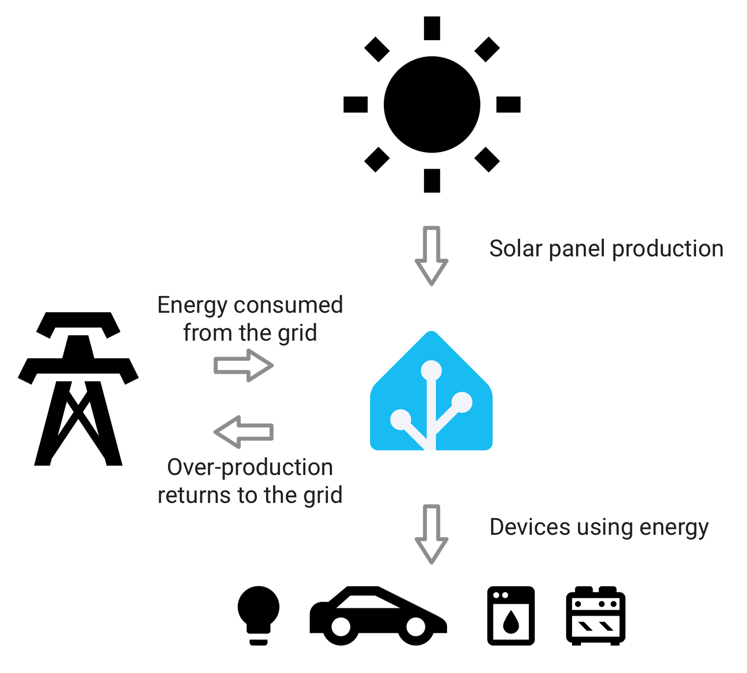
A dashboard can make patterns easier to see, but the cost analysis is only as sound as its import, export, production, tariff, and time-zone configuration.
Check weekday and weekend patterns separately
An hourly average across the whole month can hide the reason for a spike. Split the analysis at least four ways:
- weekday versus weekend;
- occupied versus regularly unoccupied days;
- mild versus hot or cold days;
- solar-producing versus low-solar days, if relevant.
For industry users, this segmentation is important before recommending hardware. A stable daily peak suggests an automatable or scheduled load. A weather-linked peak points toward building performance, HVAC controls, or equipment efficiency. A pattern limited to a few unusual days may not justify a permanent metering expansion.
Turn findings into a seven-day experiment
Do not change five habits at once. Choose one recurring cost block and run a controlled test.
- Select one or two expensive hours that occur on several comparable days.
- Identify one flexible load likely to contribute.
- Record the baseline cost for that hour across the previous week.
- Shift or reduce only that load for seven days.
- Compare kWh and cost for the same hour and similar day types.
- Check whether usage moved to a cheaper interval or merely returned later at the same price.
- Keep the change only if the saving is repeatable and the household can live with it.
Good first experiments include delaying a dishwasher, moving EV charging, reviewing a pool-pump schedule, testing a hot-water control window, or reducing an unnecessary overnight load. For practical appliance timing, see Best Time to Run Dishwasher, Washing Machine, and Dryer on Time-of-Use.
When smart meter data is not enough
Utility interval data shows when the property imported or exported energy. It usually does not prove which device caused the interval.
Add faster or more granular monitoring when:
- several large loads overlap inside each interval;
- you need live feedback rather than next-day data;
- a battery, EV charger, solar diverter, or automation requires local control;
- the site needs circuit-level attribution;
- three-phase behaviour is being hidden by a net total;
- the data portal does not offer a usable export.
A whole-home monitor can narrow the time window, while circuit meters or plug-in meters can attribute individual loads. Start with the billing-boundary data first, then add sensors only where the remaining uncertainty affects a decision. The article Is a Whole-Home Energy Monitor Worth It? helps decide whether that extra layer is justified.
Common analysis mistakes
Avoid these before acting on the results:
- comparing bill dollars without normalising for the number of days;
- using kW as though it were interval kWh;
- assigning one tariff rate to every interval on a time-of-use plan;
- ignoring seasonal, weekend, public-holiday, or controlled-load rules;
- mixing import and export into a single unsigned value;
- treating estimated or missing intervals as measured behaviour;
- shifting loads to “off-peak” without checking the current plan;
- assuming the biggest one-off spike is the largest monthly cost opportunity;
- ignoring demand charges when the bill includes them;
- changing the tariff before testing whether the household can actually shift demand.
A monthly review that takes 15 minutes
Once the spreadsheet is built, repeat this short review each billing cycle:
- Compare average kWh per day with the previous bill and the same season last year.
- List the five highest-cost hours of day.
- Check whether weekday and weekend rankings changed.
- Review the overnight minimum and evening peak.
- For solar, compare midday export with later import.
- Note tariff or feed-in-rate changes before comparing cost.
- Choose one experiment for the next month.
This is more useful than chasing every short spike. It keeps attention on patterns that can change a bill.
Final recommendation
Use smart meter data as a cost map. Convert each interval into money using the tariff that actually applied, group costs by hour, and look for repeated high-cost blocks rather than dramatic single events.
For most households, the best first target is a flexible load that overlaps an expensive period: EV charging, clothes drying, dishwashing, water heating, pool equipment, or avoidable heating and cooling overlap. For solar homes, also test whether those loads can move into real surplus-solar hours.
The result should be a small number of specific actions, not a more complicated dashboard. If the interval data identifies the costly hour but cannot identify the load, that is the point where faster whole-home or circuit-level monitoring earns its place.